Replication of Schmitt-Grohé and Uribe (2003)
Closing Small Open Economy Models

This report was created as part of the assessment for the Computational Economics Course in the PhD program at Collegio Carlo Alberto taught by Florian Oswald.
Introduction
This project replicates the results of:
Schmitt-Grohé, S. and Uribe, M. (2003),
Closing Small Open Economy Models,
Journal of International Economics, 61, 163–185. https://www.sciencedirect.com/science/article/abs/pii/S0022199602000569
The paper studies alternative methods for closing small open economy models and compares their quantitative implications for business cycle dynamics and second moments.
The project reproduces the main model specifications presented in the paper using Julia and the MacroModelling.jl package. In particular, we replicate the impulse response functions and unconditional second moments for Models 1 to 4.
In addition, we extend the original analysis by implementing Model 5 under perfect foresight and studying the effects of alternative terminal conditions on the transitional dynamics of the economy.
The implementation is partly based on the Dynare replication files provided by Johannes Pfeifer: https://github.com/JohannesPfeifer/DSGE_mod/tree/master/SGU_2003
High Level Description of Computational Problem
Models 1–4
The first four models in Schmitt-Grohé and Uribe (2003) study alternative methods for inducing stationarity in small open economy models with incomplete international financial markets.
All models share the same core RBC structure and are subject to stochastic productivity shocks:
\[ a_t = \rho a_{t-1} + \sigma \varepsilon_t \]
where \(a_t\) denotes total factor productivity and \(\varepsilon_t \sim \mathcal{N}(0,1)\).
The models mainly differ in the mechanism used to stabilize foreign debt dynamics:
- Model 1: endogenous country risk premium;
- Model 1a: endogenous discount factor;
- Model 2: debt-elastic interest rate premium;
- Model 3: portfolio adjustment costs;
- Model 4: complete asset markets benchmark.
Households solve a standard intertemporal optimization problem subject to budget and capital accumulation constraints. The equilibrium conditions include Euler equations such as:
\[ \lambda_t = \beta (1+r_t)\mathbb{E}_t[\lambda_{t+1}] \]
together with labor supply conditions and aggregate resource constraints.
From a computational perspective, the problem consists of:
- computing the deterministic steady state;
- linearizing the equilibrium conditions around steady state;
- solving the resulting rational expectations system;
- simulating the model after a productivity shock;
- computing impulse response functions and unconditional second moments.
In our replication, Models 1 to 4 are implemented in Julia using the MacroModelling.jl package. The package automatically processes the DSGE model equations and computes a first-order perturbation approximation around the steady state. The resulting linearized model is then used to generate impulse response functions and simulated moments.
The implementation closely follows the Dynare replication files by Johannes Pfeifer, which were used as a benchmark for calibration choices and shock normalization.
Model 5: Perfect Foresight Computation
Unlike the previous models, Model 5 does not include a mechanism that induces stationarity in foreign debt dynamics. To study the transitional dynamics after a productivity shock, we solve the model under perfect foresight over a finite horizon.
The economy is initialized at the deterministic steady state and agents are assumed to perfectly anticipate the future path of the economy after the realization of the shock. The solution therefore consists of computing the entire transition path of the endogenous variables simultaneously.
The dynamic structure of the model is characterized by a set of nonlinear equilibrium conditions, including the intertemporal Euler equation,
\[ \lambda_t = \beta (1+r)\lambda_{t+1}, \]
the capital accumulation equation,
\[ k_{t+1} = (1-\delta)k_t + i_t, \]
and the external resource constraint,
\[ c_t + i_t + d_t = y_t + (1+r)d_{t-1}. \]
Given initial conditions and a path for productivity, the unknown sequences for consumption, investment, capital, labor, debt, and marginal utility are stacked into a large nonlinear system covering all periods of the simulation horizon.
The system is solved numerically using the NLsolve.jl package.
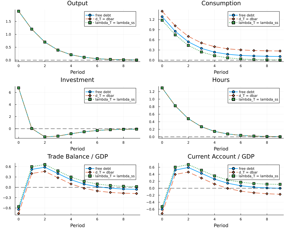
Since Model 5 is non-stationary, the finite-horizon solution depends on the terminal conditions imposed at the end of the simulation. We compare three alternative specifications:
- free terminal debt drift;
\[ d_T = d_{T-1} \]
- debt converging toward steady state;
\[ d_T = \bar d \]
- convergence of capital and marginal utility toward steady state;
\[ k_{T+1} = k^{ss}, \qquad \lambda_T = \lambda^{ss} \]
The comparison highlights how terminal conditions mainly affect intertemporal variables such as debt dynamics, consumption, and the current account, while real variables such as output and labor remain relatively similar across specifications.
Our Computational Setup
The project was developed and executed locally using both Julia and Dynare.
The computations were performed on the following systems:
- Mac Laptop M2 MacBook Air, MacOS 15.6.1, 8 GB of memory, (M2 Processor, 8 cores)
- Mac Laptop M4 MacBook Air, MacOS 15.7.7, 16 GB of memory, (M4 Processor, 10 cores)
The main software and packages used in the project are:
- Dynare (version 6.5)
- Julia (version 1.12.4)
- MacroModelling.jl
- NLsolve.jl
All package versions and dependencies are fully documented in the Project.toml and Manifest.toml files included in the repository, ensuring computational reproducibility.
Results
Models 1–4: Replication
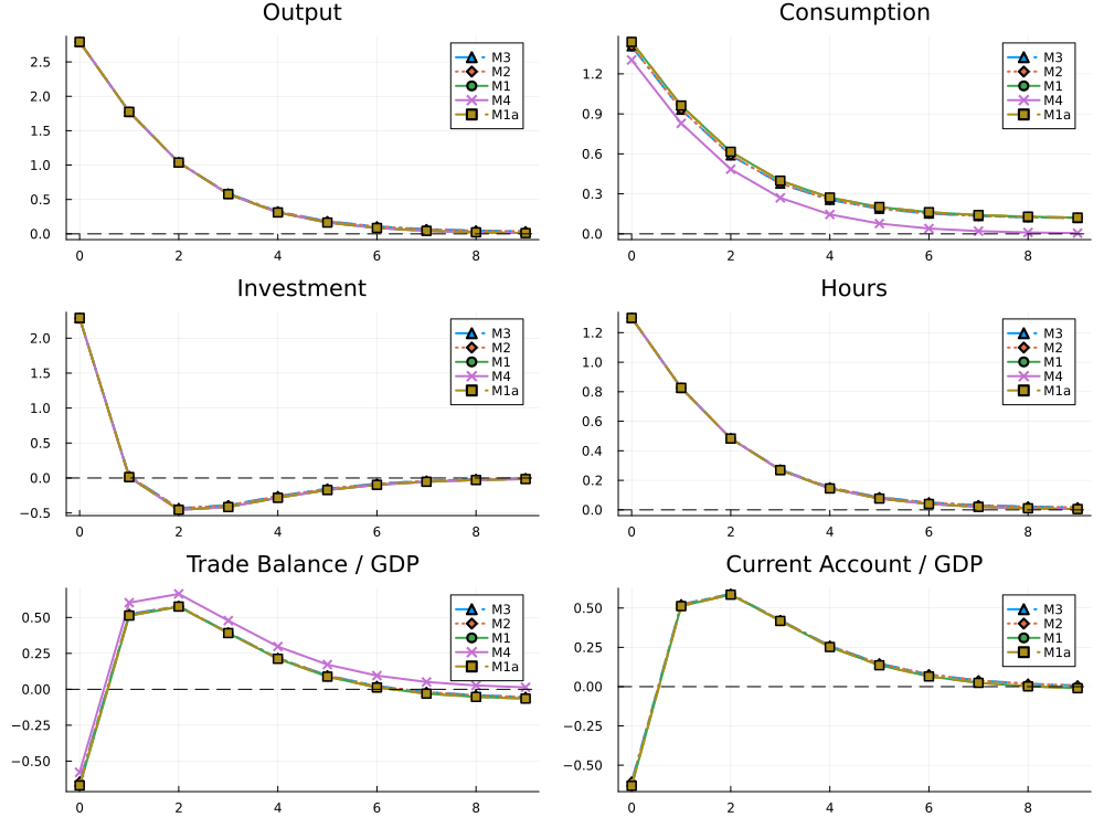
For Models 1–4, we reproduce the main impulse response functions and second moments using MacroModelling.jl.
IRFs Reported in Schmitt-Grohé and Uribe (2003)
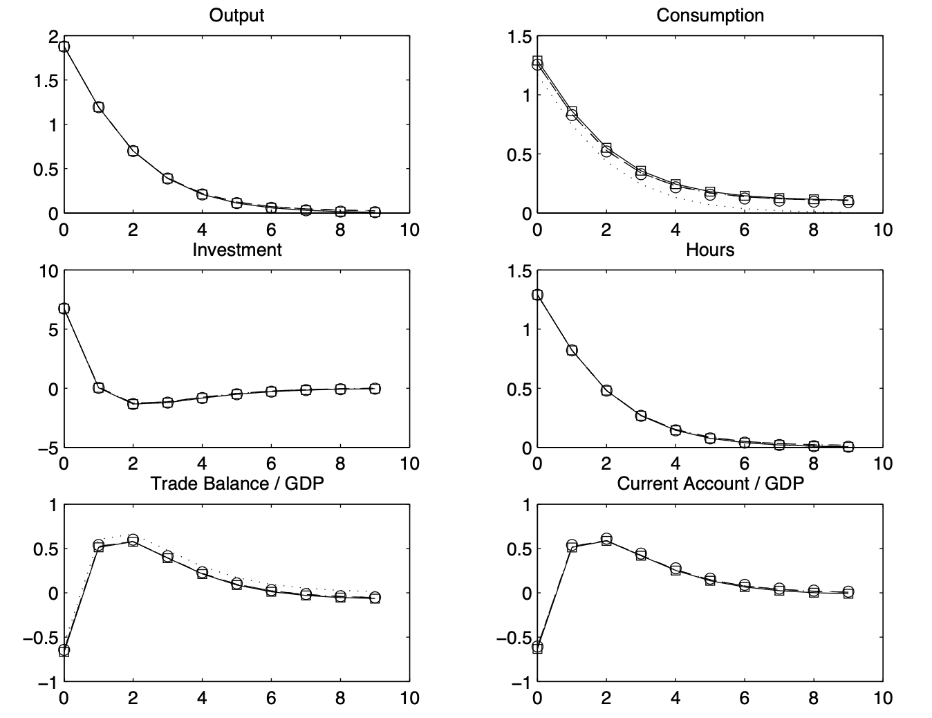
Note. Solid line: Endogenous discount factor model; Squares: Endogenous discount factor model without internalization; Dashed line: Debt-elastic interest rate model; Dash-dotted line: Portfolio adjustment cost model; Dotted line: complete asset markets model; Circles: Model without stationarity inducing elements.
Replicated IRFs
Moments Reported in Schmitt-Grohé and Uribe (2003)
| Moment | Model 1 | Model 1a | Model 2 | Model 3 | Model 4 |
|---|---|---|---|---|---|
| Volatilities | |||||
| std(\(y_t\)) | 3.1 | 3.1 | 3.1 | 3.1 | 3.1 |
| std(\(c_t\)) | 2.3 | 2.3 | 2.7 | 2.7 | 1.9 |
| std(\(i_t\)) | 9.1 | 9.1 | 9.0 | 9.0 | 9.1 |
| std(\(h_t\)) | 2.1 | 2.1 | 2.1 | 2.1 | 2.1 |
| std(\(tb_t/y_t\)) | 1.5 | 1.5 | 1.8 | 1.8 | 1.6 |
| std(\(ca_t/y_t\)) | 1.5 | 1.5 | 1.5 | 1.5 | |
| Serial Correlations | |||||
| corr(\(y_t,y_{t-1}\)) | 0.61 | 0.61 | 0.62 | 0.62 | 0.61 |
| corr(\(c_t,c_{t-1}\)) | 0.70 | 0.70 | 0.78 | 0.78 | 0.61 |
| corr(\(i_t,i_{t-1}\)) | 0.07 | 0.07 | 0.069 | 0.069 | 0.07 |
| corr(\(h_t,h_{t-1}\)) | 0.61 | 0.61 | 0.62 | 0.62 | 0.61 |
| corr(\(tb_t/y_t,(tb/y)_{t-1}\)) | 0.33 | 0.32 | 0.51 | 0.50 | 0.39 |
| corr(\(ca_t/y_t,(ca/y)_{t-1}\)) | 0.30 | 0.30 | 0.32 | 0.32 | |
| Correlations with Output | |||||
| corr(\(c_t,y_t\)) | 0.94 | 0.94 | 0.84 | 0.85 | 1.00 |
| corr(\(i_t,y_t\)) | 0.66 | 0.66 | 0.67 | 0.67 | 0.66 |
| corr(\(h_t,y_t\)) | 1.00 | 1.00 | 1.00 | 1.00 | 1.00 |
| corr(\(tb_t/y_t,y_t\)) | -0.012 | -0.013 | -0.044 | -0.043 | 0.13 |
| corr(\(ca_t/y_t,y_t\)) | 0.026 | 0.025 | 0.050 | 0.051 |
Replicated Moments
| Moment | Model 1 | Model 1a | Model 2 | Model 3 | Model 4 |
|---|---|---|---|---|---|
| Volatilities | |||||
| std(\(y_t\)) | 3.07 | 3.07 | 3.08 | 3.08 | 3.07 |
| std(\(c_t\)) | 2.35 | 2.35 | 2.71 | 2.68 | 1.91 |
| std(\(i_t\)) | 9.1 | 9.1 | 9.04 | 9.04 | 9.1 |
| std(\(h_t\)) | 2.11 | 2.11 | 2.12 | 2.12 | 2.11 |
| std(\(tb_t/y_t\)) | 1.55 | 1.55 | 1.78 | 1.76 | 1.58 |
| std(\(ca_t/y_t\)) | 1.46 | 1.46 | 1.45 | 1.45 | |
| Serial Correlations | |||||
| corr(\(y_t,y_{t-1}\)) | 0.61 | 0.61 | 0.62 | 0.62 | 0.61 |
| corr(\(c_t,c_{t-1}\)) | 0.7 | 0.7 | 0.78 | 0.78 | 0.61 |
| corr(\(i_t,i_{t-1}\)) | 0.07 | 0.07 | 0.07 | 0.07 | 0.07 |
| corr(\(h_t,h_{t-1}\)) | 0.61 | 0.61 | 0.62 | 0.62 | 0.61 |
| corr(\(tb_t/y_t,(tb/y)_{t-1}\)) | 0.32 | 0.32 | 0.51 | 0.51 | 0.39 |
| corr(\(ca_t/y_t,(ca/y)_{t-1}\)) | 0.3 | 0.3 | 0.32 | 0.32 | |
| Correlations with Output | |||||
| corr(\(c_t,y_t\)) | 0.94 | 0.94 | 0.84 | 0.85 | 1.0 |
| corr(\(i_t,y_t\)) | 0.66 | 0.66 | 0.67 | 0.67 | 0.66 |
| corr(\(h_t,y_t\)) | 1.0 | 1.0 | 1.0 | 1.0 | 1.0 |
| corr(\(tb_t/y_t,y_t\)) | -0.02 | -0.01 | -0.04 | -0.04 | 0.13 |
| corr(\(ca_t/y_t,y_t\)) | 0.03 | 0.03 | 0.05 | 0.05 |
Model 5: Perfect Foresight Extension
Perfect Foresight IRFs
Discussion
The short-run responses of output, investment, and hours are almost identical across the three cases, since they are mainly driven by the common technology shock and the production side of the model. The differences are more visible for consumption, the trade balance, and the current account.
This is the key point of the non-stationary benchmark. Since Model 5 does not include a debt-elastic interest rate, portfolio adjustment costs, or any other stationarity-inducing mechanism, foreign debt is not forced to return to its steady-state level. As a result, the computed transition path depends on how the finite-horizon problem is closed.
Hence, for the non-stationary model, impulse responses are not completely independent of the chosen terminal condition. The computational closure affects the economic interpretation of the adjustment dynamics.